Extremely Fast and Succinct RMQ with Wide Segment Trees
This note describes several advanced techniques for static RMQ, where the array is known in advance and does not change, but the queries are not known ahead of time. The goal is to build two succinct RMQ variants:
- one that uses \(1.05n\) auxiliary bits and sometimes accesses the original array;
- one that uses \(2.1n\) auxiliary bits and never accesses the original array.
Both implementations are fast in practice, reaching roughly \(20\) to \(30\) ns on average for uniformly random queries over arrays of about \(10^9\) elements.
For comparison, the Codeforces tutorial on block-based RMQ reports roughly \(100\) ns per query on arrays of length \(10^7\) with 32-bit integers, while using 32 auxiliary bits per entry.
AI disclosure
AI was extensively use for text writing, coding, experimentation and image generation for this article. Author (Nikolay Malkovsky) takes full responsibility for the content and possible mistakes/inaccuracies.
Block-Based RMQ
We use the following formulation. Given an array \(A[0..n-1]\), construct a data structure that can answer this query quickly:
\[ RMQ(l, r) = \arg \min_{i \in [l, r)} A[i] \]
Many practical RMQ data structures use sparse tables as one component; see the cp-algorithms sparse table article for details.
The idea is simple: for each position \(i\), precompute \(RMQ(i, i + 2^k)\) for all \(k\) such that \(i + 2^k \leq n\). To answer \(RMQ(l, r)\), choose \(k\) such that \(2^k \leq r - l < 2^{k+1}\) and compare the minima from the two overlapping intervals \(RMQ(l, l + 2^k)\) and \(RMQ(r - 2^k, r)\).
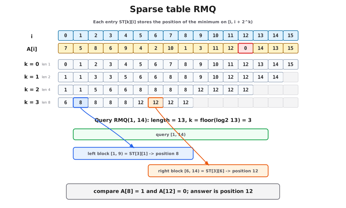
Sparse tables are good both in theory and in practice, but their \(\mathcal{O}(n \log n)\) memory usage limits practical applications. For example, for 64-bit integers, sparse tables exceed typical L3 cache sizes at around \(10^5\) elements. To scale further, we use blocking: split the array into blocks of size \(b\), solve RMQ over whole blocks with a sparse table, and then adjust the answer by solving the boundary parts inside the affected blocks.
The classical \(\mathcal{O}(n)\)-space, \(\mathcal{O}(n)\)-construction, \(\mathcal{O}(1)\)-query solution to LCA by Farach-Colton and Bender (Bender and Farach-Colton 2000) uses exactly this kind of blocking. It takes \(b = \frac{\log_2 n}{2}\) and precomputes every possible query inside a single block. A query spanning several blocks then needs two table lookups for the boundaries and one sparse-table query for the middle; a query inside one block needs only the precomputed block table. Practical solutions use the same shape, but often solve boundary and block-internal queries differently; see the Codeforces tutorial on block-based RMQ for one practical walkthrough.
Notes on Memory Access Patterns
The main problem when solving RMQ on long arrays is memory access: RAM is much slower than processor cache and quickly becomes the bottleneck. For sparse tables, for example, cache misses become visible once the table grows past cache capacity.
There is still an interesting observation about sparse tables. For uniformly random queries, about half of the intervals have length at least \(n/2\), so they are answered from the highest sparse-table levels. If levels are stored together, this layout can reduce cache misses. As a result, a sparse table over \(10^7\) elements can still answer random queries in roughly \(20\) to \(30\) ns on average even though the full table occupies several gigabytes.
Base Optimizations
Prefix/Suffix Minima Encoding
We start from the optimization described in the Codeforces tutorial on block-based RMQ.
The idea is to precompute answers for prefixes of a block. These answers form a sequence of record minima: scan the elements left to right and store the position whenever a new minimum appears. The answer to the query \([0, r)\) is then the last stored position smaller than \(r\), which can be found with a binary search. For example, for the input array \([5, 2, 7, 1, 6, 3, 4, 8]\), the sequence of prefix minima positions is \([0, 1, 3]\).
Suffixes use the same logic. For short sequences, the best encoding is a bitmask. Moreover, for a sequence of length \(n\), a single \(n\)-bit mask can encode both prefix and suffix minima. To answer prefix/suffix queries from this mask, the only extra information we need is the global minimum position \(m\):
- For prefix \([0, r)\), mask out bits at positions at least \(\min(r, m + 1)\) and find the highest set bit in the result.
- For suffix \([l, n)\), mask out bits at positions below \(\max(l, m)\) and find the lowest set bit in the result.
Here is a visual depiction of this prefix/suffix mask layout and how different query modes are answered for the input array \(A = [5, 2, 7, 1, 6, 3, 4, 8]\):
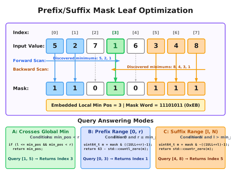
This information is not enough to answer arbitrary block-internal queries. One possible solution is to store these masks for every position, but that is overkill. For now, we first check whether an internal query contains the block minimum position; on a miss, we simply do a linear scan over the original array. The mask needs \(n\) bits and we additionally need the minimum position; a natural packed layout is therefore \(248 + 8\) bits. Later we describe how this can be generalized to \(2n\) bits while supporting block-internal queries.
Speculative Covering Interval Optimization
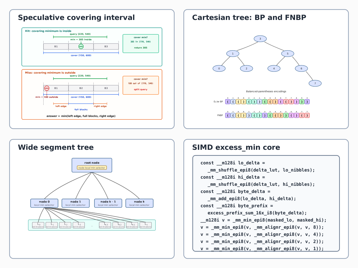
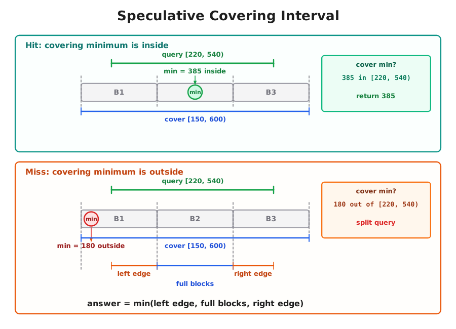
With a block-based approach, a query is usually split into three parts: the left boundary, the middle full blocks, and the right boundary. If the query lies inside a single block, it becomes one block-internal query instead. This split is often heavier than necessary, so we can apply a speculative covering interval check, following the practical covering-range idea used by Kowalski and Grabowski in Faster Range Minimum Queries (Kowalski and Grabowski 2017):
- Find the minimal block range \([B_L, B_R)\) that fully covers the query range \([l, r)\).
- Retrieve the precomputed global minimum position \(p\) for this covering block range.
- If \(l \le p < r\), return \(p\) immediately.
- If \(p\) falls outside \([l, r)\), do the normal splitting.
This early-stop optimization is highly effective for large arrays.
Cartesian Tree
The next important object is the Cartesian tree. It is built from an array as follows: the minimum is the root, and the left and right subtrees are built recursively from the left and right subarrays. Here is an example for the array \([5, 2, 7, 1, 6, 3, 4, 8]\):
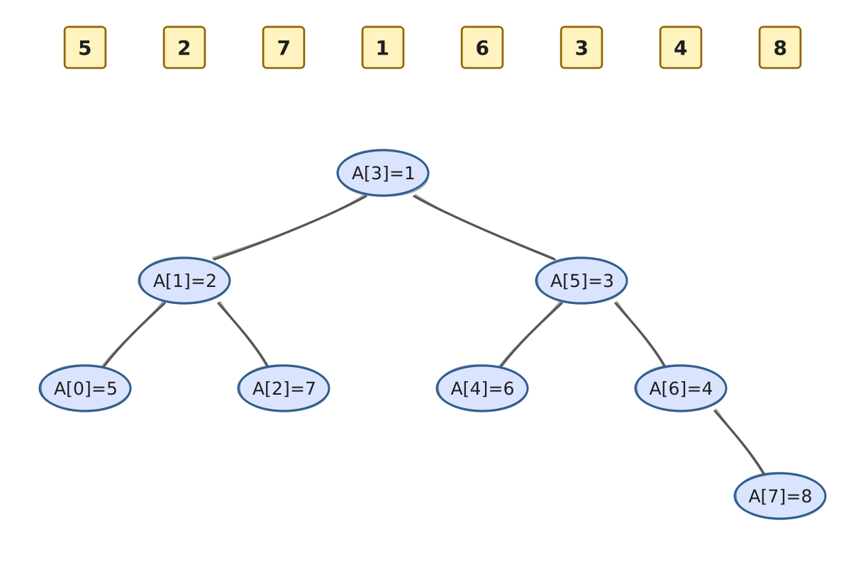
Cartesian trees are important for RMQ because RMQ reduces to LCA in the Cartesian tree. They are also connected to the prefix/suffix minima discussed above: those minima correspond to the leftmost and rightmost paths in the tree.
The standard way to solve LCA is to reduce it further to \(RMQ \pm 1\). Perform a DFS traversal, output the current depth on every move, and store the first visit time of each node. The LCA of two nodes is then the node at the minimum depth between their first visits. The key property of this RMQ instance is that adjacent depths differ by exactly \(1\). The classical Farach-Colton and Bender approach (Bender and Farach-Colton 2000) exploits this property and achieves \(O(n)\) preprocessing time and \(O(1)\) query time with Four Russians-style tables for block-internal queries. The algorithm is described in detail in e-maxx/cp-algorithms.
What matters more here is that this depth-style \(RMQ \pm 1\) instance can be encoded as a compact binary string: 0 for a \(-1\) change and 1 for a \(+1\) change.
- In fact, Cartesian-tree reduction is the route to a \(2n\)-bit-per-value RMQ encoding.
- SIMD bit manipulation can be used to accelerate queries on Cartesian trees with \(64\) to \(256\) nodes.
This note does not cover the full Cartesian-tree reduction. For the SIMD part, we are interested in the following problem. Given a binary sequence \(B:\{1, \ldots, n\}\rightarrow \{0, 1\}\), define excess as \(E_B:\{0, \ldots, n\}\rightarrow \mathbb{Z}\):
\[ E_B[i] = \sum_{j=1}^i 2B[j]-1, \]
We want to find the first position attaining \(\min E_B\) on a short range. Be slightly careful with indexing: if the bit interval is \([l, r)\), the prefix-excess positions we compare are \(l, l+1, \ldots, r\). Position \(l\) is the depth before consuming the first bit of the query, and position \(p+1\) is the depth after consuming bit \(p\).
Succinct Variant of the Cartesian Tree
An FCB-style approach would construct an Euler tour over this tree. Its succinct variant is the standard balanced-parentheses representation: perform a DFS, write ( when going down, and write ) when going up. Although this representation is sufficient, there is a better variant for RMQ. Let FNBP(node) be the corresponding sequence rooted at node. For a node with left and right children, the representation is:
"(" FNBP(left child of node) ")" FNBP(right child of node)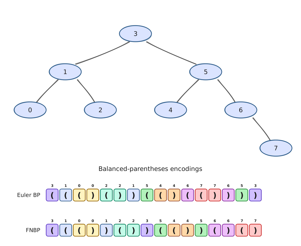
This is the Ferrada-Navarro balanced-parentheses representation from Ferrada and Navarro (2017).
There are two advantages of this representation:
- It can be constructed in a linear scan.
- The closing-parenthesis correspondence is also linear: the \(i\)-th
)corresponds to the \(i\)-th element of the array.
The key observation for answering queries in this representation is that, to get the LCA of two nodes, we need to find the leftmost position with minimum excess between the closing parentheses of the two nodes. That position is right next to the LCA’s closing parenthesis. Conversion from array position \(i\) to the position of its closing parenthesis is done by select0(i + 1), i.e. “find the position of the \((i+1)\)-st 0”. Conversion back from a close-parenthesis position to the array position is done by rank0(pos) - 1, i.e. “count the number of 0 bits before this position and convert from one-based to zero-based indexing”. For short sequences, these operations can be implemented efficiently with modern CPU instructions: POPCNT for rank, and TZCNT plus PDEP for select. For long sequences, practical implementations usually use sampling.
The FNBP sequence for a Cartesian tree can be constructed with a simple backward scan and a stack.
auto bp_sequence = ...;

for (size_t i = n; i-- > 0;) {
  while (!stack.empty() && A[stack.back()] >= A[i]) {
    stack.pop_back();
    prepend_open(bp_sequence);  // '('
  }

  stack.push_back(i);
  prepend_close();   // ')', one per array entry
}

while (bp.size() != 2 * n) {
  prepend_open(bp_sequence);    // final unmatched stack entries
}
Every array entry emits exactly one closing parenthesis when it is pushed. Since the scan goes right-to-left and every emitted bit is prepended, these closings appear in the final BP sequence in the same order as the array entries. Thus the closing parenthesis for entry i is exactly select0(i + 1). Opens encode the nesting caused by stack pops and the final cleanup; closes identify the array positions.
For the example array, the FNBP sequence is:
bp position:   0  1  2  3  4  5  6  7  8  9 10 11 12 13 14 15
paren:         (  (  (  )  )  (  )  )  (  (  )  )  (  )  (  )
excess:     0  1  2  3  2  1  2  1  0  1  2  1  0  1  0  1  0
array index:            0  1     2  3        4  5     6     7
To answer a query on a range [l, r), convert l and r - 1 to their ) positions, find the minimum excess between these positions, and convert back:
first_close = select0(l + 1)
last_close  = select0(r)
depth query = [first_close + 1, last_close + 2)
answer      = rank0(excess_min(depth query).position) - 1
For the rest of this section, use the value-RMQ query [0, 6) as an example. It maps to:
first_close = select0(0 + 1) = 3
last_close  = select0(6)     = 11
depth query = [4, 13)
For short BP blocks, select0 does not need a full sampled index. If the block fits in one 64-bit word, the position of the one-based k-th zero can be found with PDEP and TZCNT:
uint64_t zeros = ~word & valid_bits_mask;
uint64_t selected = _pdep_u64(1ull << (k - 1), zeros);
uint32_t pos = _tzcnt_u64(selected);
Here zeros marks the close parentheses. PDEP deposits the single source bit 1 << (k - 1) into the k-th set position of zeros; TZCNT then converts that one-hot mask back to a bit position. select1 is the same operation with word instead of ~word. For a short 128-bit block, do this on the first word if it contains enough zeros, otherwise subtract its zero count and continue in the second word.
Finding the minimum excess is more involved: it uses several parallel table lookups. In the walkthrough below we keep the 16-bit example, while the natural implementation unit is a 128-bit SIMD register.
The 16 bits are split into four 4-bit chunks.
chunk index:   0     1     2     3
positions:     0..3  4..7  8..11 12..15
bits:          1110  0100  1100  1010
For each 4-bit chunk, we store three lookup-table values:
delta      = total excess change after all 4 bits
local_min  = minimum excess after consuming at least one bit in the chunk
offset     = first local prefix offset 1..4 attaining local_min
chunk: 0 1 2 3
bits: 1110 0100 1100 1010
local prefixes: 1,2,3,2 -1,0,-1,-2 1,2,1,0 1,0,1,0
delta: +2 -2 0 0
local_min: +1 -2 0 0
offset: 1 4 4 2The query [4, 13) starts at nibble 1 and ends after the first bit of nibble 3. The scalar chunk calculation uses the exclusive prefix sum of delta as the base excess before each chunk, then ignores inactive chunks and uses a partial lookup for the right boundary chunk:
chunk:            0     1     2     3
active bits:      -  0100  1100     1
base excess:      -    +2     0     0
candidate value:  -     0     0     1
candidate pos:    -     8    12    13
Now do the same computation in the deinterleaved SIMD layout. A 128-bit block is loaded as bytes; each byte contributes one low and one high nibble:
byte lane:     0     1
low nibble:   1110  1100     // nibble indices 0, 2
high nibble:  0100  1010     // nibble indices 1, 3
In code this is:
const __m128i excess_lut_nibble_mask_sse = _mm_set1_epi8(0x0F);
const __m128i excess_lut_delta_sse = _mm_setr_epi8(
    -4, -2, -2,  0, // 0000 0001 0010 0011
    -2,  0,  0,  2, // 0100 0101 0110 0111
    -2,  0,  0,  2, // 1000 1001 1010 1011
     0,  2,  2,  4  // 1100 1101 1110 1111
);

const __m128i bytes = _mm_loadu_si128(reinterpret_cast<const __m128i*>(s));
const __m128i lo_nibbles =
    _mm_and_si128(bytes, excess_lut_nibble_mask_sse);
const __m128i hi_nibbles =
    _mm_and_si128(_mm_srli_epi16(bytes, 4), excess_lut_nibble_mask_sse);
Here excess_lut_nibble_mask_sse is a 16-byte SSE register where every byte is 00001111 (0x0F). The first and extracts the low 4-bit chunk from every input byte. For the high chunks, _mm_srli_epi16(bytes, 4) shifts each 16-bit lane right by four bits; the second and then removes the neighboring byte bits that entered during that 16-bit shift, leaving again one clean nibble value in each byte lane. These byte values are now valid indices in [0, 15] for _mm_shuffle_epi8 LUT lookups.
excess_lut_delta_sse is the 16-entry table for the total excess change of a 4-bit chunk. A 1 bit contributes +1, and a 0 bit contributes -1, so the entry is
delta[nibble] = 2 * popcount(nibble) - 4For example, nibble 0000 has delta -4, nibble 0001 has delta -2, nibble 0111 has delta +2, and nibble 1111 has delta +4. The table is stored in nibble-index order because _mm_shuffle_epi8(table, nibbles) treats each byte of nibbles as a table index and returns the corresponding delta.
The delta lookup is aligned with the byte lanes. The low nibbles hold chunk indices 0 and 2; the high nibbles hold chunk indices 1 and 3:
byte lane:      0      1
low bits:    1110   1100
low code:       7      3
lo_delta:      +2      0

high bits:   0100   1010
high code:      2      5
hi_delta:      -2      0

byte_delta:     0      0   // lo_delta + hi_delta
These values are computed with table lookups:
const __m128i lo_delta = _mm_shuffle_epi8(excess_lut_delta_sse, lo_nibbles);
const __m128i hi_delta = _mm_shuffle_epi8(excess_lut_delta_sse, hi_nibbles);
const __m128i byte_delta = _mm_add_epi8(lo_delta, hi_delta);
The prefix scan is now over byte deltas, not nibble deltas. Lane i of byte_prefix stores the excess after byte i. The following code is a standard way to compute prefix sums over bytes in a 16-byte array. Each shift propagates partial sums from distances 1, 2, 4, and 8 bytes:
static inline __m128i excess_prefix_sum_16x_i8(__m128i v) noexcept {
  v = _mm_add_epi8(v, _mm_slli_si128(v, 1));
  v = _mm_add_epi8(v, _mm_slli_si128(v, 2));
  v = _mm_add_epi8(v, _mm_slli_si128(v, 4));
  v = _mm_add_epi8(v, _mm_slli_si128(v, 8));
  return v;
}
In this example, only the first two bytes are populated. Since both bytes have net delta 0, the inclusive prefix sum is also zero in both lanes:
byte_prefix:         [ 0, 0 ]
byte_prefix_before:  [ 0, 0 ]
byte_prefix means “the excess after this byte”. In general, for byte_delta = [d0, d1, d2, ...] we get:
byte_prefix:         [d0, d0+d1, d0+d1+d2, ...]
byte_prefix_before:  [ 0,    d0,    d0+d1, ...]
byte_prefix_before is produced by shifting byte_prefix by one byte and inserting zero in lane 0. We need this “before” value because the low nibble of each byte starts at the byte boundary, and the high nibble starts after the low nibble, so its base is byte_prefix_before + lo_delta.
const __m128i byte_prefix = excess_prefix_sum_16x_i8(byte_delta);
const __m128i byte_prefix_before = _mm_slli_si128(byte_prefix, 1);
The next table lookup returns the local minimum inside each full 4-bit block. The table excess_lut_min_sse is organized like delta: the input nibble is an index, and the result is the minimum local excess reached after reading at least one bit of that nibble.
__m128i lo_local_min = _mm_shuffle_epi8(excess_lut_min_sse, lo_nibbles);
__m128i hi_local_min = _mm_shuffle_epi8(excess_lut_min_sse, hi_nibbles);
Real query boundaries rarely coincide with 4-bit boundaries. In the actual implementation, boundary nibbles are easier to handle separately: either with a small scalar table, or with the same table plus an active-position mask. The SIMD middle then receives only full 4-bit blocks. In this example, the left boundary already coincides with the start of block 1, while the right boundary cuts block 3 down to its first bit. To keep the walkthrough in one place, we substitute the partial value +1 for block 3 instead of using the full value for nibble 1010.
lo_local_min:       [ +1, 0 ]     // 1110 has min +1; 1100 has min 0
hi_local_min full:  [ -2, 0 ]     // 0100 has min -2; 1010 has min 0
hi_local_min used:  [ -2,+1 ]     // block 3 only uses its first bit: 1
The low nibble starts at the byte boundary and uses byte_prefix_before as its base. The high nibble starts after the low nibble, so its base also includes lo_delta:
lo_candidates = byte_prefix_before + lo_local_min
              = [0, 0] + [1, 0]
              = [1, 0]

hi_candidates = byte_prefix_before + lo_delta + hi_local_min
              = [0, 0] + [2, 0] + [-2, +1]
              = [0, 1]
const __m128i lo_candidates =
_mm_add_epi8(byte_prefix_before, lo_local_min);
const __m128i hi_candidates =
_mm_add_epi8(_mm_add_epi8(byte_prefix_before, lo_delta), hi_local_min);Now we remove inactive blocks from consideration. Conceptually, the active part of the query [4, 13) is:
chunk:                 0       1        2       3
bits:               1110    0100     1100    1010
active part:           -    0100     1100       1
Inactive candidates are replaced with the sentinel value 127. This is larger than any excess inside a 128-bit block, so it cannot become the minimum:
masked_lo = [127, 0]
masked_hi = [  0, 1]
First compare the low and high 4-bit-block candidate inside each byte lane:
pairwise_min = min(masked_lo, masked_hi)
             = [0, 0]
Then reduce the 16 signed byte lanes to one scalar minimum. Here _mm_alignr_epi8(v, v, shift) is used as a byte rotation of the same register. After comparisons with shifts 8, 4, 2, and 1, every byte lane contains the minimum over the original 16 lanes, so we can read lane 0.
v = _mm_min_epi8(v, _mm_alignr_epi8(v, v, 8));
v = _mm_min_epi8(v, _mm_alignr_epi8(v, v, 4));
v = _mm_min_epi8(v, _mm_alignr_epi8(v, v, 2));
v = _mm_min_epi8(v, _mm_alignr_epi8(v, v, 1));
candidate_min = static_cast<int>(
    static_cast<int8_t>(_mm_extract_epi8(v, 0)));
In this example:
candidate_min = 0Now we need the first 4-bit block that attains this minimum. We compare masked_lo and masked_hi with candidate_min, convert the result to bit masks with movemask, take the first set bit, and map the byte lane back to the 4-bit-block index:
masked_lo == 0: [false, true ]  => low byte 1  => block index 2
masked_hi == 0: [true,  false]  => high byte 0 => block index 1
first winning block index = min(2 * 1, 2 * 0 + 1) = 1
Finally, the offset table gives the first local position of the minimum inside the winning block. The important convention is that local_offset is in the range 1..4: it is not the bit index inside the block, but the excess position after reading that many bits. For block 1, namely 0100, the local minimum -2 is reached for the first time after four bits.
excess position = 4 * block_index + local_offset
                = 4 * 1 + 4
                = 8
This is the first interior zero-depth position in the BP sequence. In the query [4, 13), position 12 also attains depth 0, but first-minimum tie-breaking keeps position 8. Therefore RMQ(0, 6) returns rank0(8) - 1 = 3, which is the position of A[3] = 1.
For a short BP block, rank0(pos) is just a masked popcount over the zero bits before pos:
static inline uint32_t rank0_u64(uint64_t word, uint32_t pos) noexcept {
  uint64_t before = pos == 64 ? ~uint64_t{0} : ((uint64_t{1} << pos) - 1);
  return std::popcount((~word) & before);
}
For pos = 8, the mask keeps BP bits 0..7; four of them are zero, so rank0(8) = 4 and the array position is 4 - 1 = 3.
Wide Segment Tree
The final detail needed for the RMQ solution is the wide segment tree. See Sergey Slotin’s Algorithmica article on segment trees (Slotin 2022) for a detailed explanation. The general idea is that a regular segment tree is binary and does not fully use SIMD parallelism or cache-line-wide memory accesses. A B-tree variant decreases the height of the tree without a large increase in per-node CPU work, because the node-local work can be handled with SIMD operations.
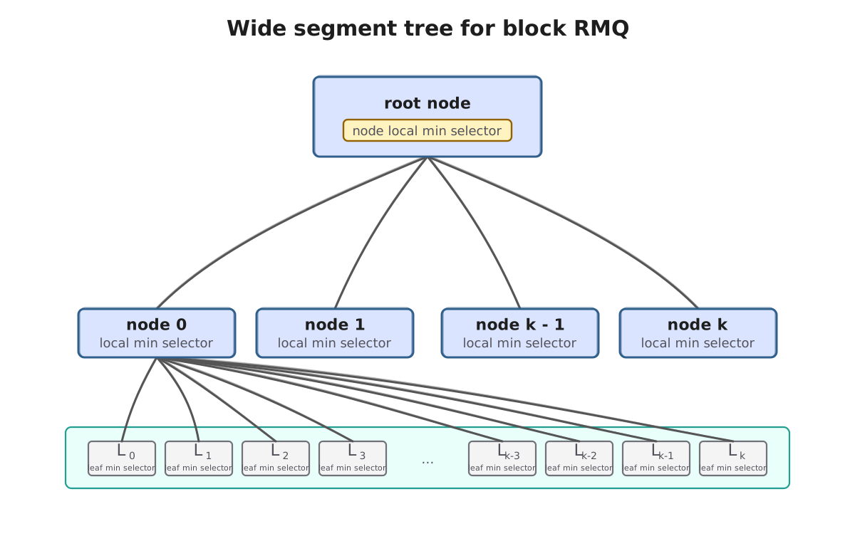
We add an important improvement for RMQ. In the original approach, the node fanout \(B\) is derived so that \(B\) values fit into the target SIMD register or cache line. For RMQ, we can instead store a node-local Cartesian tree over the child minima. This lets us increase the fanout to \(B=256\), for which the local Cartesian tree fits into 64 bytes.
Final Solutions
We now have two solution variants using the ideas above. The first variant occasionally accesses the original array:
- For each block of \(L=496\) entries, construct a prefix/suffix mask with a 16-bit minimum position.
- Construct sparse tables over blocks of size \(S\). Choose \(S\) so that the table occupies only a few megabytes and comfortably fits in L3 cache.
- Construct a wide segment tree over blocks of size \(L\) with fanout \(256\), and store a Cartesian tree inside each node for fast minimum extraction.
The query is answered as follows:
- First find a covering segment of \(S\) blocks and query the sparse table. If the returned position lies inside the original query, return it.
- On a sparse-table miss, choose the minimum among three candidates: the left boundary \(S\) block, the middle subsegment of full \(S\) blocks, and the right boundary \(S\) block.
- Boundary blocks are answered with the wide segment tree; the middle subsegment is answered with the sparse table.
- Prefix/suffix queries on \(L\) blocks are answered with the precomputed mask. For internal queries, fall back to a linear scan over the original array.
The second variant is similar, but builds a global Cartesian tree so that queries do not need to access the original array.
The following plot shows timings for the hybrid variants on fully random queries over the available benchmark sizes:
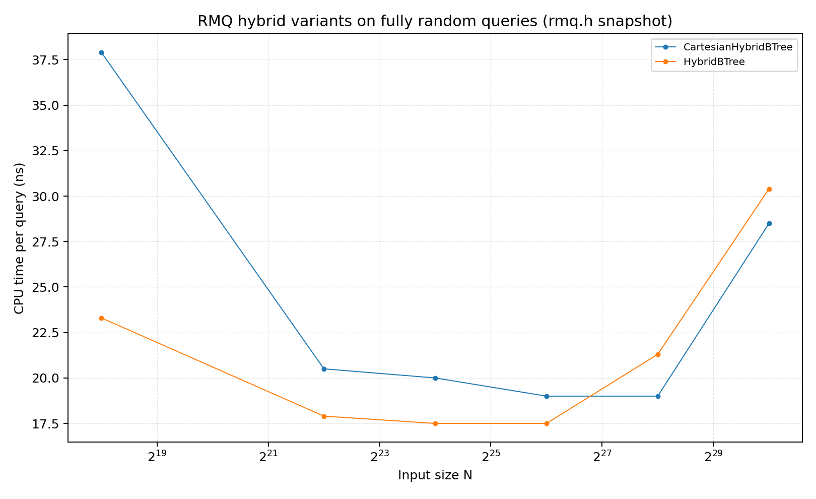
The final implementations are available in Pixie (Malkovsky 2026), the entry point is the RMQ header include/pixie/rmq.h, corresponding two implementations are classes HybridBTree and CartesianHybridBTree.
Pixie disclaimer
I’m working on succinct data structure library pixie, If I got your interest and you want to collaborate – feel free to contact me.